
What is a Box Cox Transformation?
- Data transforms are usually applied so that the data appear to more closely meet assumptions of a statistical inference model to be applied or to improve the interpret-ability or appearance of graphs.
- Power transformation is a class of transformation functions that raise the response to some power. For example, a square root transformation converts X to X1/2
- Box Cox transformation is a popular power transformation method developed by George E. P. Box and David Cox.
Box Cox Transformation Formula
The formula of the Box Cox transformation is:
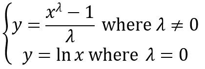
Where:
- y is the transformation result
- x is the variable under transformation
- λ is the transformation parameter
Use Minitab to Perform a Box-Cox Transformation
Minitab provides the best Box-Cox transformation with an optimal λ that minimizes the model SSE (sum of squared error). Here is an example of how we transform the non-normally distributed response to normal data using Box-Cox method.
Data File: “Box-Cox” tab in “Sample Data.xlsx”
Step 1: Test the normality of the original data set.
- Click Stat → Basic Statistics → Normality Test.
- A new window named “Normality Test” pops up.
- Select “Y” as “Variable.”
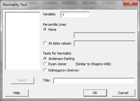
- Click “OK.”
- The normality test results are shown automatically in the new window.
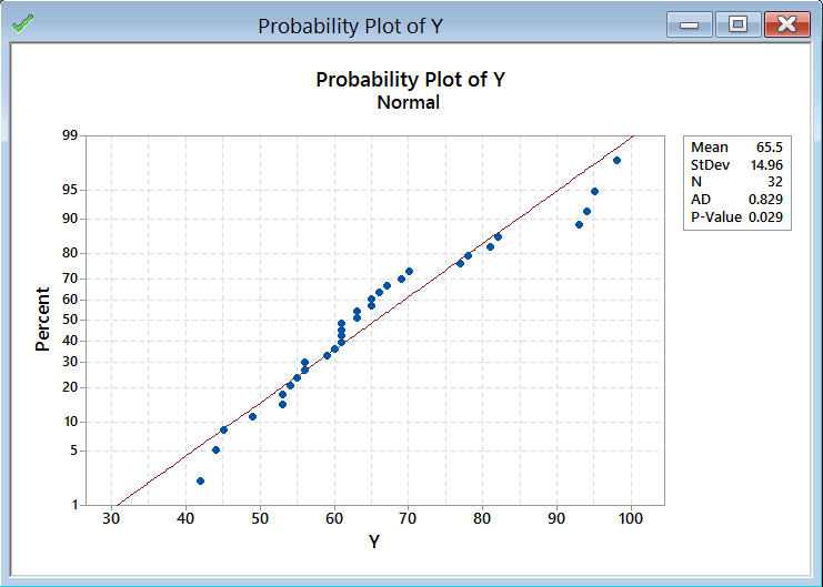
Normality Test:
- H0: The data are normally distributed.
- H1: The data are not normally distributed.
If p-value > alpha level (0.05), we fail to reject the null hypothesis. Otherwise, we reject the null. In this example, p-value = 0.029 < alpha level (0.05). The data are not normally distributed.
Step 2: Run the Box-Cox Transformation:
- Click Stat → Control Charts → Box-Cox Transformation.
- A new window named “Box-Cox Transformation” pops up.
- Click into the blank list box below “All observations for a chart are in one column.”
- Select “Y” as the variable.
- Select “Run” into the box next to “Subgroup sizes (enter a number or ID column).”
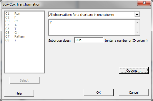
- Click “OK.”
- The analysis results are shown automatically in the new window.
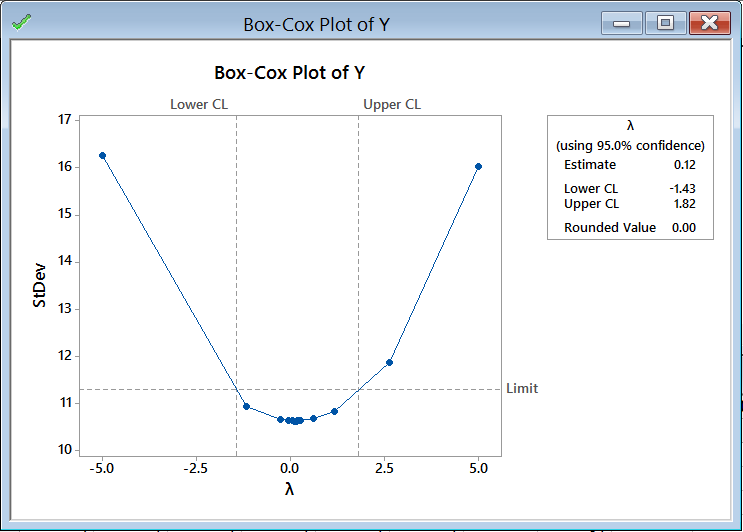
The software looks for the optimal value of lambda that minimizes the SSE (Sum of Squares of Error). In this case the minimum value is 0.12. The transformed Y can also be saved in another column.
- Create a new column named “Y1” in the data table.
- Click Stat → Control Charts → Box-Cox Transformation.
- Again, a window named “Box-Cox Transformation” pops up.
- Like before, Select “Y” as the variable.
- Select “Run” into the box next to “Subgroup sizes (enter a number or ID column).”
- Now, click on the “Options” button in the “Box-Cox Transformation” window.
- A new window named “Box-Cox Transformation – Options” appears.
- Click in the blank box under “Store transformed data in” and all the columns pop up in the list box on the left.
- Select “Y1” in “Store transformed data in.”
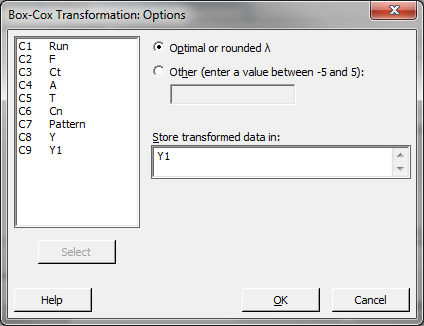
- Click “OK” in the window “Box-Cox Transformation – Options.”
- Click “OK” in the window “Box-Cox Transformation.”
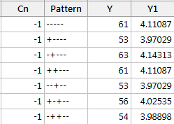
- The transformed column is stored in the column “Y1.”
Run the normality test to check whether the transformed data are normally distributed.
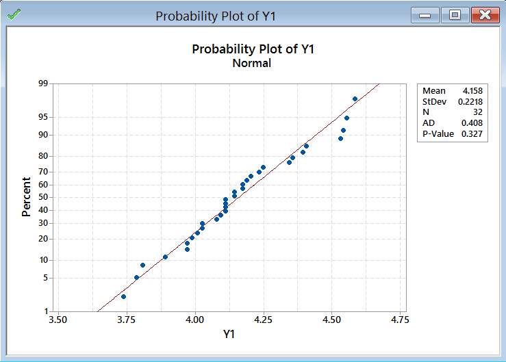 Use the Anderson–Darling test to test the normality of the transformed data
- H0: The data are normally distributed.
- H1: The data are not normally distributed.
Model summary: If p-value > alpha level (0.05), we fail to reject the null. Otherwise, we reject the null. In this example, p-value = 0.327 > alpha level (0.05). The data are normally distributed.
Comments are closed.