Chi Square Test with JMP

Chi Square (Contingency Tables)

We have looked at hypothesis tests to analyze the proportion of one population vs. a specified value, and the proportions of two populations, but what do we do if we want to analyze more than two populations? A chi-square test is a hypothesis test in which the sampling distribution of the test statistic follows a chi-square distribution when the null hypothesis is true. There are multiple chi-square tests available and in this module we will cover the Pearson’s chi square test used in contingency analysis.

• Null Hypothesis (H₀): p₁ = p₂ =… = p_k
• Alternative Hypothesis (H_a): At least on of the proportions is different from others.

The symbol k is the number of populations of our interest; k ≥ 2.

What is the Chi Square Test?

The chi-square test can also be used to test whether two factors are independent of each other. In other words, it can be used to test whether there is any statistically significant relationship between two discrete factors.

• Null Hypothesis (H₀): Factor 1 is independent of factor 2.
• Alternative Hypothesis (H_a): Factor 1 is not independent of factor 2.

Chi Square Test Assumptions

• The sample data drawn from the populations of interest are unbiased and representative.
• There are only two possible outcomes in each trial for an individual population: success/failure, yes/no, and defective/non-defective etc.
• The underlying distribution of each population is binomial distribution.
• When np ≥ 5 and np(1 – p) ≥ 5, the binomial distribution can be approximated by the normal distribution.

How Chi Square Test Works

Test Statistic

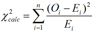
Where:

• Oi is an observed frequency
• Ei is an expected frequency
• N is the number of cells in the contingency table.

If (calculated chi-square statistic) is smaller than (critical value), we fail to reject the null hypothesis. The test statistic is calculated with the observed and expected frequency.

Use JMP to Run a Chi-Square Test

Case study 1: We are interested in comparing the product quality exam pass rates of three suppliers A, B, and C using a nonparametric (i.e. distribution-free) hypothesis test: chi-square test.

Data File: “Chi-Square Test1” tab in “Sample Data.xlsx”

• Null Hypothesis (H0): pA = pB = pC
• Alternative Hypothesis (Ha): At least one of the suppliers has different pass rates from the others.

Steps to run a chi-square test in JMP:

1. Click Analyze -> Fit Y by X

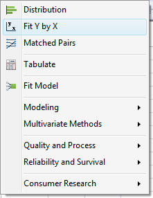
Fig 1.1 Analyze>Fit Y by X

2. Select “Results” as “Y, Columns”
3. Select “Supplier” as “X, Factor”
4. Select “Count” as “Freq”

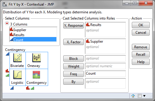
Fig 1.2 Distribution for Y and X

5. Click “OK”

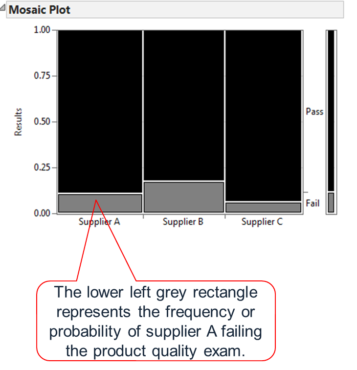
Fig 1.3 JMP Mosaic Plot results

Mosaic plot is a graphical tool to divide the frequency data into smaller segments each of which is represented by a rectangle with the area proportional to the frequency of a specific outcome.

• The Y axis displays the classification of response. In our example, Y has two possible values: pass or fail.
• The X axis displays the different levels of a factor “Supplier”.
  A contingency table displays the results for each supplier. It helps us to understand how the counts translate to percentages of the column, row, and grand total number of observations.

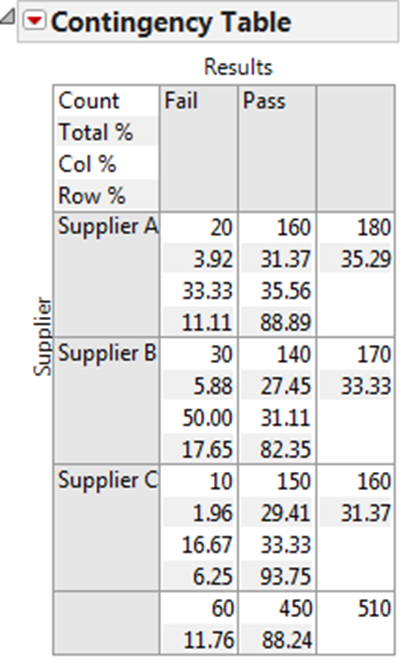
Fig 1.4 Contingency Table result per supplier

To see more statistics in the contingency table, click on the red triangle button next to “Contingency Table” and select the statistic of interest.

Case study 2: We are trying to check whether there is a relationship between the suppliers and the results of the product quality exam using nonparametric (i.e. distribution-free) hypothesis test: chi-square test.

Data File: “Chi-Square Test2” tab in “Sample Data.xlsx”

• Null Hypothesis (H0): Product quality exam results are independent of the suppliers.
• Alternative Hypothesis (Ha): Product quality exam results depend on the suppliers.

Steps to run a chi-square test 2 in JMP:

1. Click Analyze -> Fit Y by X

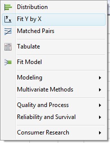
Fig 2.1 Analyze>Fit Y by X

2. Select “Results” as “Y, Columns”
3. Select “Supplier” as “X, Factor”
4. Select “Count” as “Freq”

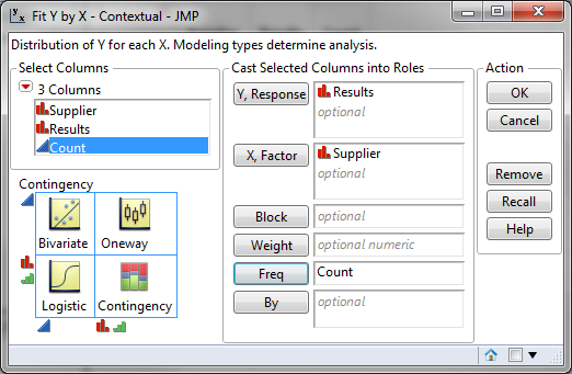
Fig 2.2 Distribution for Y and X

5. Click “OK”

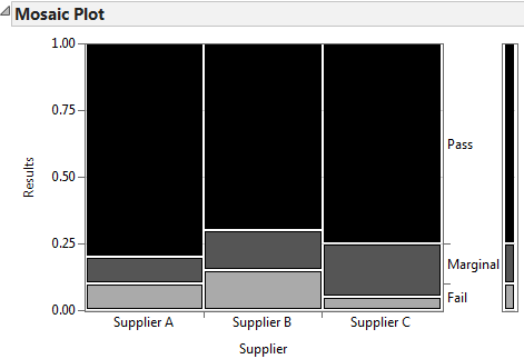
Fig 2.3 Mosaic Plot output

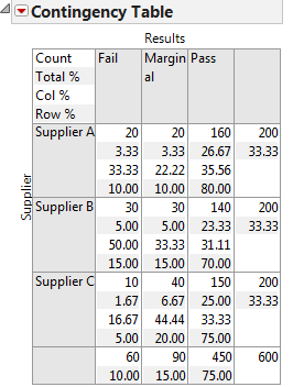
Fig 2.4 Contingency Table output

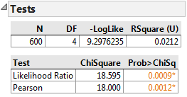
Fig 2.5 Chi-Square test results
The p-value is smaller than the alpha level (0.05) and we reject the null hypothesis. The product quality exam results are not independent of the suppliers. These results indicate the danger that we can get into when using discrete data. Not everything is as simple as yes/no or pass/fail. Even though supplier C has a lower fail rate of 10, you can see that the number of marginal results is higher. However, the p-value tells us that we must reject the null hypothesis and claim that the quality exam results are dependent on the suppliers.